My teammates Evan Smith, Helen Heimark, and Hannah Parker are the members of Group 3 and as of now, we have completed nine (9) different experimental lab activities/subjects; of which five (5) different lab reports have been produced & submitted. These nine experiments were as follow:
Overall, I've been neutral in my opinions about each lab however, I do believe that for a one credit hour course, we have to dedicate a lot of time and effort to complete each assignment; it should be worth 2-3 credit hours if you ask me.
TENSILE TEST
During this lab, we used three different apparatus: Q-Test machine, Extensometer, and Test works software platform. We were also given five plastic specimens, along with one aluminum specimen; each had their width and thickness measured & recorded. Once it was time to load the specimens into the jaws of the Q-Test machine, we then measured the grip separation. Then, the test was ran on each specimen while the software recorded the numerical data and saved it to our flash drives. In the end, each specimen broke in half as shown in Figure 1. Finally, we collected our data, performed our calculations of the stress-strain relationship for the two different materials (polymers and metallic) and produced graphs that represented this relationship; all of which were submitted in an official lab report.

Figure 1-Tensile Test Specimen
CREEP
Before creating a lab report, we performed the experiment through the use of the SM1006 creep measurement as our apparatus. Other equipment required to carryout this lab were the VDAS Software, Vernier, weights (800gm), weight hanger, and 3D printed specimens. We learned that creep is when a material has the tendency of deforming permanently under the influence of mechanical stresses. Our main objective was to experimentally obtain the creep curve as shown in Figure 2.

Figure 2-Typical Creep Curve
Source: http://www.nptel.ac.in/courses/112107146/lects%20&%20picts/image/lect12/fig%206.jpg
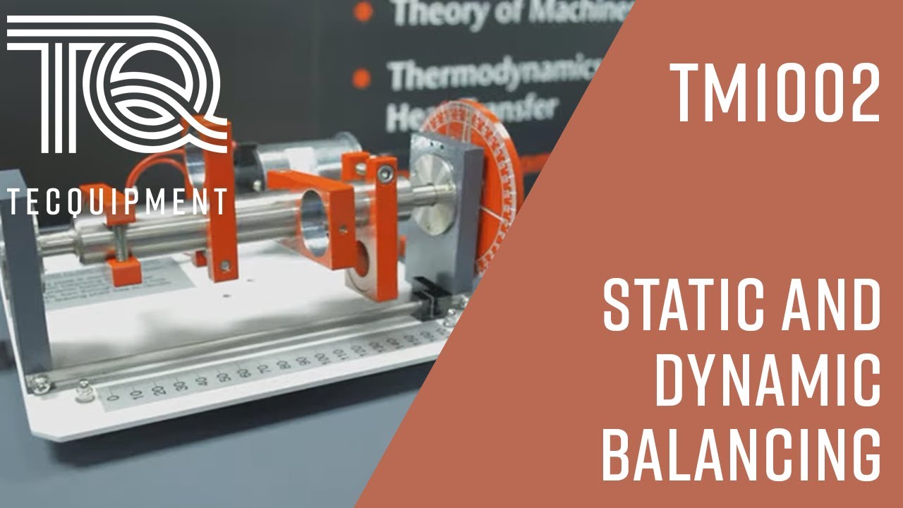
DYNAMIC BALANCING
The in-class portion of this lab consisted of the dynamic balancing experiment in which we mounted a shaft with masses on it so that it may become statically balanced and dynamically balanced. When the shaft was statically balanced, the angular position of the masses remained constant without rotating; when it was dynamically balanced on the other hand, there were no vibrations. For our experiment, we used a balanced four mass system similar to that shown in Figure 3 and completed a quick worksheet that was turned in at the end of class.

Figure 3-Balanced Four Bar System
Source: https://i.ytimg.com/vi/p1JDMvWGdsk/maxresdefault.jpg
TORSION
In this lab, we applied twist to three different materials (aluminum, brass, steel) shown in Figure 4 and measured the amount of rotation applied by the hand crank of the apparatus; the apparatus used were the TQ Torsion Testing device. We used degrees ranging from 0 to 3 to experimentally develop a method that utilized the torsion testing apparatus to determine the relationship between angles of twist and torsional load. We formally documented this experiment with a lab report.

Figure 4-Sample Materials for Torsion
FATIGUE
The fatigue experiment was one that was quickly performed in class and turned in with an associated worksheet. During this lab, we used the MT 3012-E Fatigue Testing Machine shown in Figure 5 as our apparatus to predict the fatigue life. The rest of the materials and equipment used were a brass and aluminum specimen, along with a vernier caliper. The theory behind this experiment was that rupture can be caused by a large number of stress variations at a point, even if the maximum stress hasn't reached the yield stress; this is known as the fatigue of a material.

Figure 5-MT 3012-E Fatigue Testing Machine
Source: ME350 Fatigue Tester File
BUCKLING
In our formal lap report, we determined the load-deflection function and critical loads of a sample column through an experimental method that utilized the buckling of columns apparatus (as shown in Figure 6). To determine the critical load, we used Euler's formula; to determine the maximum deflection of the column, we used the Secant formula. The width, length, and thickness of the struts (steel, aluminum, brass) were measured and recorded before they were analyzed in the pinned-pinned end-conditions.

Figure 6-Columns Apparatus for Buckling Lab
DEGREE OF FREEDOM
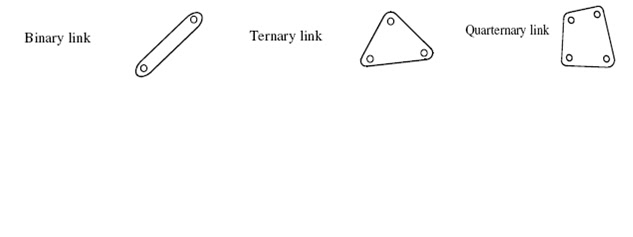
For the Degree of Freedom (DOF) lab, the instructor prepared different stations that each consisted of their own mechanisms and mobility. What we were tasked with as a group was to go around with our worksheet at each station and calculate the DOF and mobility of each system. This activity put to use the Mechanisms and Mobility Analysis lecture that we went over for Mechanisms of Machines (ME372). If the mechanism was in 2D, we used the formula:
M=3(L-1)-2J1-J2
and if the mechanism was in 3D, used the formula:
M=6(L-1)-5J1-4J2-3J3-2J4-J5
where (M) is the DOF or mobility of the mechanism, (L) the number of links— Figure 7 shows the different types of links, and the (J) the number of joints that had the specific DOF associated with the subscript.

Figure 7-Types of Links
Source: http://1.bp.blogspot.com/-x-dCQw6wmg4/TvP6IXpZkZI/AAAAAAAAAK8/EVVD_m9Qu2M/s1600/gps.bmp
BENDING
Our final lap report for the Mid-term was over our bending experiment. The main objective was calculating the deflection of the shaft from adding equal amounts of masses at an equal distance at the end of the beams; we were also asked to determine the strain at the surface of the beam. Once we analyzed our results, we noticed some error in the second part/station of the experiment. The apparatus that was used to complete the lab was the Beam Apparatus and a free-body diagram is shown in Figure 8.

Figure 8-Free Body Diagram of the Bending Lab Experiment
Source: ME350 Bending of Beams File
WHIRLING
In the whirling experiment, we simply used the TMI MKII Whirling of Shafts machine as our apparatus to get the steel shaft to form the first mode (single bow) and second mode of whirling (double bow) as shown in Figure 9. We used the formula for the fundamental frequency of transverse vibrations to calculate the theoretical frequencies. Then, we compared these results with the measured natural frequencies of the shaft which was calculated by using a digital tachometer to measure the rotational speed of the shaft. The lab was very simple and most likely my favorite one yet.

Figure 9-The First and Second Mode of Whirling
Source: https://qph.ec.quoracdn.net/main-qimg-9c0fb36366b6b11967494f294b47c246
GRAIN SIZE
The grain size experiment was an interesting one because it was the first lab that we conducted in this course where we had to use a microscope and Adobe Photoshop software to obtain our calculations. The apparatus we operated is shown in Figure 10 below; this a reflected light optical microscope called the Olympus PME3. During this lab we magnified two different specimen and took pictures that were later on used in the Adobe Photoshop tool, along with the ruler tool to calculate diameter of each grain size; the two materials that were observed were bronze and steel. Using the ASTM grain size number after performing our calculations, we later on classified whether the two materials were coarse-grained, medium-grained, fine-grained, or ultra-fine grained.

Figure 10-The Olympus PME3 Microscope
Source: ME 350 Grain Size File
STRESS CONCENTRATIONS
Stress concentration was observed through the use of a circular polariscope with either a white or a monochromatic light. The different levels of stress of the bi-refringment material had a characteristic value called a fringe value that was calculated by determine the major and minor principle stresses. To complete the worksheet that was handed out, we determined the fringe order and based off of the colors we observed. This lab was very subjective because each person identified the colors differently. Figure 11 shows the colors referenced to determine our calculations and observations.

Figure 11-Fringe Orders Based on Observed Colors
Source: ME 350 Stress Concentration File
CAM FOLLOWER
In this lab, we were originally tasked with studying the displacement, velocity, and acceleration profile of two different cams—tangent and curved cams—however, due to the design error of the tangent cam, we were only able to study the curved cam. Although we didn't mind during the lab, when it came to writing our formal report, we were unable to compare our values. For those of you who are unfamiliar, a cam is sometimes defined as a machine element or mechanism that has a curved outline or a curved groove, which oscillates or rotates and moves a separate mechanism called the follower. The TM21 Cam Analysis Machine (CAM) shown in Figure 12 below was used to obtain a sketch of the displacement.

Figure 12-TM21 Cam Analysis Machine
Source: ME 350 Cam File
GEAR TRAIN
The gear train experiment was associated with a quick worksheet we completed in class as a group. Gear trains come in many different types however, we mostly worked with a epicyclic gear train. The Sanderson Coupled Epicyclic Unit apparatus was operated in two different modes (each mode tested one at a time) so that we would calculate the angular velocity ratio and the torque ration, along with the efficiency. To be able to perform these calculations, the weight at the output shaft for each mode was recorded. Figure 13 displays an apparatus similar to the one used in class.

Figure 13-An Epicyclic Gear Train Apparatus
Source: http://discoverarmfield.com/media/filter/l/img/acceleration_geared_systems_sd1_28.jpg
HARDNESS TEST
Our last and final lab experiment required the implications of various Rockwell Hardness Test Modes as our apparatus to analyze the hardness of metal, ceramic and polymeric materials. Hardness was defined as a material's resistance to penetration. Unlike the previous lab experiments this semester, a formal lab report wasn't conducted for the experiment; instead, we turned in a worksheet during class. To complete the worksheet, five values of hardness for each test samples were obtained and compared to their actual values on their respective scales. The lab was simple and took just a few minutes to complete; within those minutes we used a 100 Kgf weight for the B scale and 150 Kgf for the C scale; the B scale was used with softer materials like aluminum, brass, and soft steels while the C scale was used with harder materials like iron & harder steels. Figure 14 displays the Rockwell Hardness Test apparatus that was operated during this experiment.

Figure 14-Rockwell Harness Tester
Source: ME 350 Rockwell Hardness Test File
MACHINE LAB TOUR
Although this section is titled "Machine Lab Tour", we were honestly introduced to mostly one machine: the milling machine. Unlike a lathes, mills keep the desired object that needs to be cut stationary while the machine part used for cutting is in motion. For the specific mill demonstrated, our instructor was simply trying to level off a block of metal scrap he found laying around the lab. He also showed us how to use the computer attached in put in the location coordinates for the specific mill used; this isn't a prominent feature in most mills. Personally, I have been introduced to milling machines before during my time as a FIRST Robotics Competition mentor where I milled my own bearings for parts of our robot. Anyway, during the tour we simply listened and didn't actually operate the machine. In the end, the instructor also informed us of how to file or remove the rough edges on the materials once we achieve the desired specifications. Figure 15 below shows an image of an average milling machine.

Figure 15-Milling Machine

 Please wait...